Tricks Island

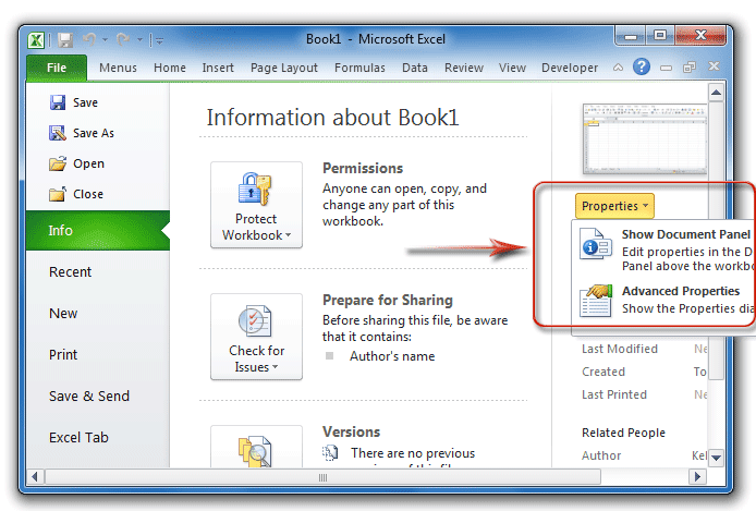
You can change a variety of workbook properties in Excel 2010.  These can include author, organisation, keywords, title or tags.  This information is sometimes referred to as metadata. 1.      Open the worksheet that you would like to change the properties of. 2.      Click the File tab and ensure Info is selected to view the workbook properties in the right-hand pane. 3.      To amend these details, click on any grey text that begins with Add a…. This will open a field for you to enter your custom information. 4.      If you would like to edit further properties, click Properties at the top and select Advanced Properties from the list. 5.      You can update properties on the Summary tab by entering new information in the fields or on the Custom tab by selecting a property Name and entering the correct text in the Value   6.      Once you have updated all the properties, click OK to close the Properties window. Click Home to return to your w

Themes are a combination of colours, fonts and effects that can be applied Excel 2010 workbooks.  You can choose to select from the predefined, built-in themes or you can also change various settings and save it as a new theme.  To find out more about the creating custom themes, see the How to Create a New Theme tutorial . 1. Open the workbook that you would like to apply the theme to. 2. On the Page Layout tab, click Themes in the Themes group to display the various themes  3. Click the theme you would like to apply to your workbook to see each element alter  NOTE: The column and row headings also change to reflect the theme. 4. To change any of the Font, Color or Effects , click the relevant category in the Themes group on the Page Layout tab and select an alternative set. That’s it for applying a Theme.  Hope you found it useful – don’t forget to take a look at our next tutorial on creating a new theme in Excel 2010! If you've any quest

When applying a theme to an Excel 2010 workbook, there may be elements you wish to amend and update.  A theme is a set of colours, fonts and effects that can be adjusted according to your requirements.  Your new updated themes can be saved for future use. 1. Open the workbook that has the theme you wish to modify applied to the contents. NOTE: If you not have a suitable workbook, open a new, blank workbook and apply a theme to it. To find out more about applying themes, see the How to apply a Theme tutorial . 2. On the Page Layout tab, in the Themes group, select either Colors, Fonts or Effects.  Choose one of the options provided. NOTE: If none of the sets are suitable for your formatting requirements, you can choose to create a custom set of colours or fonts. To do this, click the relevant option in the Themes group and select Create New Theme Fonts or Create New Theme Colors . Modify according to your requirements and save to create a new set of fonts or

Here's a quick tip that can help prevent a bit of frustration when using Excel.  Many times when you are sorting or scrolling in Excel, the column headers will move along with the rest of your data. To prevent your column headers (or really any row or column), select the row or column that comes after.  For example, to prevent the column headers in row 1 from moving: 1. Select row 2 by clicking "2" as shown in the screenshot below:Column Headers in Excel 2. With row 2 selected, go to the "Windows" menu and select "Freeze Panes"Freeze Column Headers 3. Your column header should now be locked in place and you will be able to sort and scroll without moving your column labels.  A line will show up which indicates which part of your workbook is frozen. If you've any question, problem, suggestion and feedback than please comment below. Have a nice day!

To get a list of unique values you can use the AutoFilter or you can try using a formula approach. The COUNTIF function only has two arguments, Range and Criteria.  The range would be your data range.  In the below example it’s A2:A9.  The criteria would be the value you want to count in the range.  So if we wanted to count the number of times the number 8 appeared in the data range below, the formula would be =COUNTIF(A2:A:9, 8).  This would return 3 because the value 8 occurs three times in the range specified.  Instead of setting the criteria to 8 we could point it to a cell containing that value.  So the formula would then be =COUNTIF(A2:A:9, A3).  It’s worth noting that Excel 2007/2010 has a new function called COUNTIFS which allows multiple ranges and criteria. To get the unique values in a range lets use the COUNTIF function wrapped in an IF statement.  This is called nesting.  In Excel 2003 an IF statement can have up to seven levels of nested functions.  For

What are absolute and relative references and why should I care? Well, first let’s answer what they are.  Have you ever seen an excel formula with a dollar sign ($) in it?  That’s an absolute reference.  It means that the reference to the column or row it’s in front of will never change no matter where you place the formula. For example, if I have a formula reference set to =$A$2 then no matter where I copy the formula to it will always be equaled to the value in A2.  Now if I had =$A2 and I copied the formula to cell D6 then the formula would change to =$A6.  Why does this happen?  It’s because the absolute reference is for the column only and not the row.  So it will always reference column A, but the row will change to the row of wherever the formula is being copied. If you read my article on Handy Excel Shortcuts you’ll know that you can quickly and easily add the dollar signs ($) without typing them.  When you’re entering the formula, click F4 when you’re on a cell

One of the most common questions I come across is how to get a list of unique values from a column.  There are many ways to accomplish this; probably the easiest is to use the Advanced Auto Filter. For Excel 2003, select your column you want to filter and then click Data -> Filter -> Advanced Filter.  You may get a message that Excel cannot determine which row in your list contains column labels.  This means that Excel can’t find your headers.  An easy way to get around this is to bold your row that has headers.  This will let Excel know that the bolded row is your header row. You can either filter the list in place or copy the unique values to another area in your worksheet. To copy the list in place leave everything as is and select the Unique records only check box at the bottom and click OK. To copy the unique values to another location, select the Copy to another location option, enter in a Copy to range and select the Unique records only check box at t

Excel 2010 is a powerful suite from MS Office that makes it cool to like spreadsheets again. Okay, so maybe I'm not the right person to ask about what's cool and what's on my usual Saturday night schedule. Still, I like to think that I know at least a little about Office and what makes it the easiest and best for getting things down and done  – period. When it comes to using Excel, organization is everything. That's why Excel 2010 is the most organized of the organizational tools in MS Office, and Sparklines is one of the new features in Excel 2010. With Sparklines, you can create a set of small charts in a single cell to outline patterns in the data. This lets you zero in on trends in data so that you can work more quickly and with more clarity. Along with Sparklines, Excel 2010 has a slew of new filtering enhancements to make it even easier to work with your data. A wicked little feature called Slicer lets you get a rich visualization of PivotTable an

There are a few shortcuts that I use everyday.  Excel has many keyboard shortcuts which are convenient and can save you time. This is by no means a comprehensive list, but they are the most common shortcuts. F2 – This will allow you to enter edit mode in a cell, instead of double clicking on it. F3 – This will bring up the dialog to paste the names of all the named ranges in the workbook. F4 – When you are in edit mode of a cell and your cursor is on a cell reference, this will toggle between the absolute and relative references (ie. The $ in the cell reference $A$1). F5 or Ctrl + G – This brings up the Go To dialog where you can jump to certain ranges or you can click on the Special button and then select certain cells based on a variety of choices.  For instance, you can select all the Objects in the active worksheet or you can select all the formulas that equate to errors. Ctrl + End – This will bring you to the very last cell of data.  But be careful with th